1/ General Introduction

1.1/ Introduction

The pupose of this pacakge is to provide a simple interface between the drivers of a robots and a controller based on the dynamic-graph LAAS-CNRS framework. This documentation page is therefore based on http://stack-of-tasks.github.io/documentation/e_api.html. Please visit this web site if you have code question about the LAAS packages. A talk that present this page is available here: http://replay.vidyo.tuebingen.mpg.de/replay/showRecordingExternal. html?key=KEnam4DBoewz76u

If anything is not clear in this documentation please ask Maximilien Naveau or Vincent Berenz.

1.2/ General knowledge about the dynamic graph

1.2.1/ The dynamic-graph is ... a graph

Figure 1: Example of a graph based on https://git-amd.tuebingen.mpg.de/amd-clmc/dg_demos/blob/master/python/dg_demos/filter_graph.py.

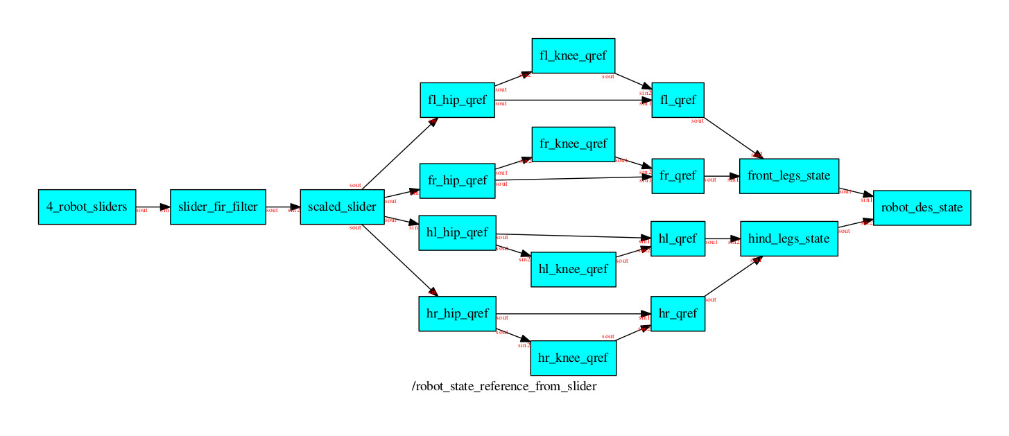
The above figure depicts a simple graph that takes as input a vector of 4 dimension containing 4 doubles (e.g. user inputs from some slider) and output a desired configuration for a quadruped robot. First step consist in filtering it and scale it to the desired reference. Then we define the hip joints to be the reference from the scaled_slider. The knee are a scaled version of the hip (knee_joint = hip_joint * (-2)). Then we concatenate the signals back to one simple vector which will be the reference state of fro a quadruped robot.

The idea of having a graph is that once a part of the graph works, it can be concatenated and can be seen as a simple node. The other powerful thing about graphs is that they can be conceptually easy to understand (not easy to use nor debug but everyone knows what a graph is ^^). The dynamic graph IS therefore a GRAPH, so it has inputs and outputs. Typically the inputs of the graph we will use are the robot sensors, and its outputs are the motor controls. Which boils down to the definition of a controller. For example, a simple graph would read the robot joint states and velocities and compute a PD controller resulting in a torque output. The concept is actually more general: A control graph is made up of no des , which consume and emit signals. For instance, it is also possible to implement a filter. Such a filter would consume the current robot state and perform a smoothing on the state measurements.

In the next section we will describe the vocabulary that is used with the dynamic-graph.

1.2.2/ A bit of vocabulary

Figure 2: This simple graph shows the vocabulary associated with the dynamic graph.

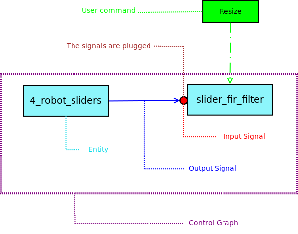
Figure 2 summarizes the different notions used in the dynamic graph. There definitions are the following:

Signals: These are arrows (see figure 1 and figure2)
Input signals: These are sockets for a node. These represent object where an output signal can be plugged in. Nodes defines only there own sockets during the setup time. output signals: These are signal emitting from a node. Nodes defines only there own output signals during the setup time.
Entity: An entity a node of the graph. Each node executes a bit of code. Control Graph: A structure of Entities and signals plugged together is a controller.
User command: A command is a non-real time punctual list of instructions. It is used to interact with entities and modify their inner states. Setup time: This is time during which the user sets up the graph. The graph IS NOT / MUST NOT BE running yet.
Plug: The fact of plugging an input signal with an output signal allow the user to define dynamically the flow of information in the graph.

1.2.3/ Typical use of the dynamic graph / Hardware communication

The "outside" of the graph is typically considered as the robot hardware. An abstraction of this "hardware", which can be virtually anything, is done by configuring the sensors and controls as signals. So in essence we create an entity that will access the hardware sensors and feed them to the graph as output signals and get back the controls as input signals. In order to configure automatically this entity we used a YAML file. We are thinking about a way to create this class from a YAML file, which would be more consistent because the urdf format is very standard.

1.3/ How does it works?

1.3.1/ The pool of entities

The dynamic graph uses the concept of singletons (https://en.wikipedia.org/wiki/Singleton_pattern):

Wikipedia definition:
In software engineering, the singleton pattern is a software
design pattern that restricts the instantiation of a class to one
"single" instance. This is useful when exactly one object is
needed to coordinate actions across the system. The term
comes from the mathematical concept of a singleton.

The concept of singleton is also useful to define a unique global variable with a specific API. Meaning that all pieces of the code can have access to the same object (a global variable), but are able to interact with it only with a specific API. The pool of entities is a singleton which manages the memory of all the entities. The pool defines each instances by an identifier (a string) and stores it.

WARNING:
Which is why one cannot create 2 entities with the same name.

The pool has therefore the capabilities of extracting the pointer to your instances and give it back to you if you lost this pointer.

WARNING:
Therefore all instances of entities can be considered as "global variables"

1.3.2/ Back propagation of the signal call

Figure 3: Zoom of the end of the graph depicted in figure 1

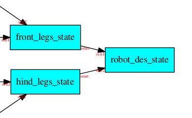
Consider the graph above (figure 3). In this graph the output signal of robot_des_state is not represented but in this particular case let us call it "sout" like "signal out". In order to execute the complete graph in figure 1 one needs to call for an update of the final output signal. Meaning that one will call:

robot_des_state.sout.recompute(current_time)

This will trigger a the evaluation of a callback method in the robot_des_ state entity if current_time>last_recomputed_time. This time management allows you to change the period of reevaluation of each signals.

Let us now assume we triggered the evaluation of robot_des_state.sout with a big enough time "T" number so the callback function is evaluated. This callback function needs to acquire the value of robot_des_state.sin1 and robot_des_state.sin2 at time T. The fact that front_legs_state.sout is plugged to robot_des_state.sin1 imply that when robot_des_state.sin1 data is accessed front_legs_state. sout will be recomputed at time T to provide the data.

INFORMATION:
Therefore the evaluation of one output signal recursively
trigger the "Left part of the graph"

1.3.3/ The concept of a command

So far the idea is that the last output signal provides the command to the robot which supposed to happen periodically. The purpose of a command is to manage asynchronous event. Typically a user command. For example on has implemented a filter like in figure 2. A user command will be helpful for 2 things:

The user needs a specific initialization, like setting the size of the filter buffer (resize command in green in figure 2).
The user needs to punctually access internal values of an entity.

In the first case the command will modify the inner structure of the entity. In the second case the command will just read the internal structure of the entity.

1.3.4/ C++ controller, but dynamic Python setup

In dynamic graph (DG) the entities are implemented using C++. So the final graph which is the controller runs all in fast C++. This is the reason why we can run it in real time on real hardware . From these C++ entities , there is an automatic way to generate corresponding python classes. These classes are then instantiated in the python interpreter to construct the control graph.

So in summary one can implement fast complex controllers with elementary blocks and prototype it in Python .

The C++ API contains C Macros that allows you to define Commands very simply. Signals are automatically bounded in Python.

1.4/ The dynamic_graph_manager

Figure 4: This picture depicts the interaction between all the component of the robot controller.

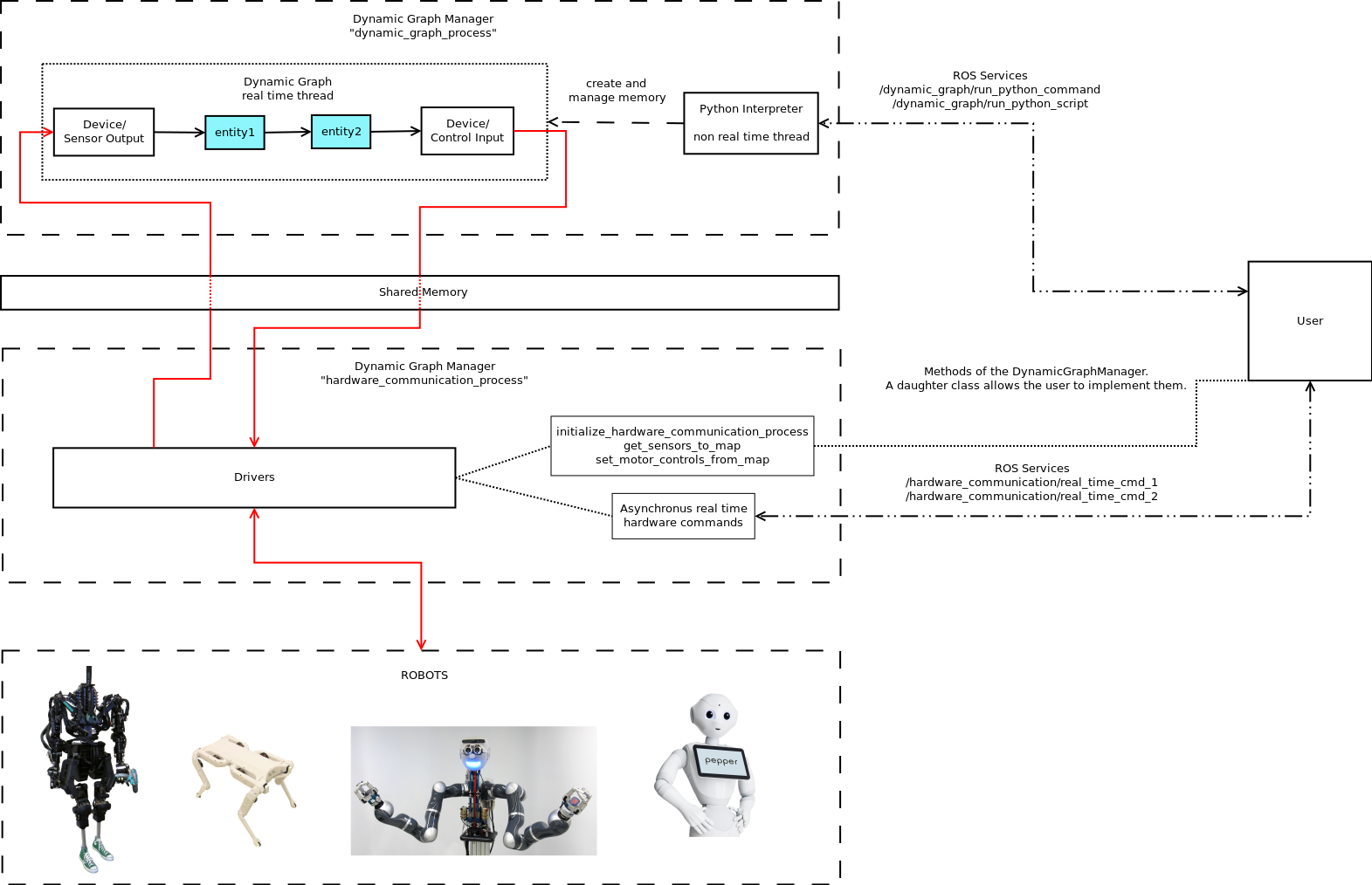
A simple demo on how to implement such a DynamicGraphManager for one robot can be seen in the demo folder of the dynamic_graph_manager package. In theses files there are examples on the creation of the DynamicGraphManager daughter class, as well as the hardware asynchronous commands and the communication with the hardware.

More details on how things are running and implemented comes in the following pages.

1.5/ Structure of the documentation

The installation procedure for this package is available here: 2/ Installation Procedure

An example to launch can be found here: 3/ Start a Dynamic Graph Manager Executable

In general this package uses one yaml configuration file to define the robot properties. A good place to store such file is a robot_properties_[robot_name] pacakge. Such packages contain urdf models, meshes, configuration files, etc. And tutorial to create such package can be found here: 4/ Implementing a robot in dynamic graph manager

This package uses the "dynamic graph" for the control. A simple example based on sot-core is available in here: 5/ Basic Control Graph

This framework lives in the ROS eco-system. So it profits from the ROS community tools such as rqt_plot, rviz. In addition to these tools a plotting tools has been develop in order to evaluate data in a dynamic way. Exmaples of usage are available here: 5/ Oscilloscope / Plotting / Logging / Motor and control process timing

Debugging the current implementationa dn specifically the dynamic graph can be tedious because of the C++/Python interaction, the spawning of different processes, etc. Exmaples of debugging technics can be found here: 6/ Debugging the implementation

In the following pages you will find how we interface the dynamic graph with a dynamical simulator: 7/ Interfacing with a robot simulator

As mention above this framework is part of the ROS eco-system. As such, the rqt framework is available. A specialization for the dynamic_graph is available as rqt_dynamic_graph. An example on how to create a robot dashboard using rqt is available here: 8/ Robot dashboard

This page present the steps executed during the continuous integration build. 9/ Continuous integration

This page shows you how to run the demo in this package. 10/ Demos

Table of Contents